Code
import IPython
IPython.display.Audio("../../data/pvqd/examples/pt0015_strain.wav")
Welcome to a blog post about exploring the Perceptual Voice Qualities Database (PVQD). This is based off of a ML + Speech workshop I held in the Berkeley Speech Group in Fall ’23. That workshop and the workbooks are available online if you want to work with the code yourself! If you’re interested in Deep Learning, there’s also some cool stuff in there about working with HuBERT representations of speech data too! The workshop doesn’t assume any knowledge of Pandas, Machine Learning, or Deep Learning, with the focus is more on getting your hands dirty with the tools vs. understanding 100% of what you’re doing.
That said, if you want to learn more about the tools, the repo contains a list of resources for learning more.
Anyways, if I’m linking to that repo, you might be wondering, why write a blog post about it? First, who doesn’t love a bit of redundancy? Second, not everyone is going to want to actually work with the code themselves. I want to communicate and share the stuff I’ve been working on, and generally share the thought processes I have when trying to work with Speech data. This is to get feedback on my work from folks who might not know a lot about data science and machine learning. This is also to serve as a type of onboarding and explanation tool for those interested in conducting voice research with publicly available datasets. Finally, I really, really need just say what I do in plain english!
And the plain English explanation is simple. Or, well, at least short. I use data science and machine learning to study voice and voice modification. I’m particularly interested in possible applications to transgender and gender-diverse voice training.
This question deserves an entire post of its own, not to mention a long discussion on the state of research in voice and voice training more generally. Still, any good tutorial requires a motivation, and the oversimplified version is this: When it comes to modifying a voice, both artificially via speech processing and physically via voice training, the current research is lacking. In speech processing, high-level modification of a particular voice is feasible, such as automatically turning a specific masculine voice into a specific feminine voice, but trying to perform lower-level modification of qualities like breathiness, strain, or resonance is either unclear or requires specialized expert knowledge. In the world of voice and voice training, research into Gender-Affirming Voice Care (GAVC) is only really starting to gain traction in Speech Language Pathology, and many of the pedagogies people pursue from online trans voice communities have not been validated experimentally or quantitatively in a formal setting. From an institutional, formal perspective, the effectiveness of behavioral voice modification, and particular approaches and pedagogies, is largely unknown.
There’s perspectives waiting to be studied, methods to be discovered, and misconceptions to be debunked. The collection and analysis of data, combined with the modeling potential of machine learning, can help in those pursuits. How? That’s a topic for a post of its own. For the time being, let’s go ahead and study some perceptual voice qualities.
Thought of as the acoustic “coloring” of an individual’s voice, perceptual qualities are one way that clinicians and voice experts conceptualize the subjective perception of a voice. Here, we provide examples of the CAPE-V perceptual qualities we use in our work. For a description of the gendered perceptual qualities of resonance and weight, we recommend taking a look over voice examples from the Voice Resource Repository by SumianVoice.
Talking about perceptual qualities in the abstract is good and all, but if you want to actually understand anything related to voice, you’re going to need to listen to them. While the CAPE-V protocol is a helpful rubric for working perceptual qualities related to vocal health, most of the voice data and assessments are privately held by voice clinics to protect the privacy of patients. Fortunately, there are a few publicly available datasets like the Perceptual Voice Qualities Database (PVQD) that contain voice samples and expert-provided ratings. In this tutorial, we’ll explore the PVQD and the CAPE-V perceptual qualities!
Here’s a list of examples of the perceptual qualities from the PVQD and their definitions per the CAPE-V Protocol.
Strain: Perception of vocal effort (hyperfunction).
import IPython
IPython.display.Audio("../../data/pvqd/examples/pt0015_strain.wav")Loudness: Deviation in perceived loudness typical for that speaker’s age and gender.
import IPython
IPython.display.Audio("../../data/pvqd/examples/pt008_loud.wav")Roughness: Perceived irregularity in the voicing source.
import IPython
IPython.display.Audio("../../data/pvqd/examples/pt0014_rough.wav")Breathiness: Audible air escape in the voice.
import IPython
IPython.display.Audio("../../data/pvqd/examples/pt118_breath.wav")Pitch: Deviation in pitch values typical for that speaker’s age and gender.
import IPython
IPython.display.Audio("../../data/pvqd/examples/pt019_pitch.wav")If you’re interested in doing anything with data, you’re going to need a way to look at it and mess wtih it. In the world of Python, one way to do that is with Pandas and Seaborn. Pandas for manipulating the data and getting it in the format you want, and Seaborn for quickly visualizing it. These are great tools for Exploratory Data Analysis (EDA), which, to butcher it with my own paraphrased phrasing, is the process of getting to know your data and understanding what possible patterns might be there. EDA is its own exciting research field, and doing it robustly requires a lot of thought about the sort of questions you’re asking. For the purposes of this tutorial, knowing that Pandas and Seaborn are two tools for performing exploratory data analysis is good enough background to get started looking at the PVQD.
If you’re interested in studying how voice varies across demographics and vocal health, the PVQD is a great starting point. Not only does the dataset contain ~2hrs of audio from vastly different speakers, the data also comes with demographic information about the speakers as well. Let’s visualize that now.
import numpy as np
import pandas as pd
import matplotlib.pyplot as plt
import seaborn as sns
plt.rcdefaults() # Default
demo_df = pd.read_csv("../../data/pvqd/pvqd_demographics.csv")
demo_df.head(5)| Participant ID | Gender | Age | Diagnosis | |
|---|---|---|---|---|
| 0 | BL01 | M | 46 | NaN |
| 1 | BL02 | F | 76 | NaN |
| 2 | BL03 | F | 88 | NaN |
| 3 | BL04 | F | 42 | NaN |
| 4 | BL05 | F | 75 | NaN |
We see that the PVQD comes with three pieces of demographic information: the participants’ Gender, Age, Diagnosis. Frustratingly as someone interested in studying transgender and gender-diverse voices, there aren’t that many datasets out there that contain more inclusive labels of gender. Gender, in the vast majority of datasets, is listed as a binary “F” or “M”. In addition to binary labels of gender, from my personal experience, most of publicly available speech datasets do not contain non-cisgender speakers. For the construction of machine learning models that can provide feedback on gender affirming voice training, this is a huge limitation. Machine learning methods often fail to generalize to unseen data, especially when that data is “out of distribution”.
Although we won’t be able to get a complete map of what voice is capable of, we can start to get a rough one. The nice thing about the PVQD is that it does provide us with voices that do exhibit certain qualities we might want to avoid during voice training, such as breathiness and strain. Let’s load in that data while we’re talking about it:
pq_train = pd.read_csv("../../data/pvqd/train_test_split/y_train.csv", index_col=0)
pq_train.head(5)| File | Breathiness | Loudness | Pitch | Roughness | Strain | |
|---|---|---|---|---|---|---|
| 0 | LA7005 | 7.000000 | 7.333333 | 7.000000 | 8.500000 | 8.000000 |
| 1 | PT116 | 31.833333 | 12.333333 | 6.000000 | 29.500000 | 7.333333 |
| 2 | PT034 | 43.166667 | 26.666667 | 61.166667 | 34.000000 | 30.333333 |
| 3 | SJ6006 | 4.375000 | 5.125000 | 0.250000 | 3.750000 | 6.875000 |
| 4 | PT005 | 5.500000 | 7.000000 | 12.000000 | 3.833333 | 4.500000 |
As we said before, the CAPE-V measures perceptual qualities on a 1-100 scale. Since these values are the average of six different raitngs, we get all those decimal places. It’s nice to look at the data like that, to make sure it’s there, but we’re still a bit away from actually learning anything about the data. I’m brushing this part under the rug (see the workshop if you’re curious!), but I’m going to clean up the data and combine the two dataframes so we can start drawing some connections.
### Fix up the demo_df first
## Fix Gender
cor_gender = {
"f": "F",
"m": "M",
"female": "F",
"male": "M"
}
demo_df["Gender"] = demo_df["Gender"].str.lower().map(cor_gender)
## Make Binary Value for Diagnosis
# Create a function to apply to the column
def process_diagnosis(diagnosis):
if pd.isnull(diagnosis):
return np.nan
if diagnosis == "N":
return "N"
else:
return "Y"
demo_df["Diagnosis "] = demo_df["Diagnosis "].map(process_diagnosis)
## We can't visualize nan data, so let's not consider those rows
# ~ is a way to invert a numpy array/pandas series of boolean values. A handy trick
diagnosis_df = demo_df[~pd.isnull(demo_df["Diagnosis "])]
# Rename column and remote white space
diagnosis_df = diagnosis_df.rename(columns={"Participant ID ": "File"})
diagnosis_df["File"] = diagnosis_df["File"].str.upper().str.strip()
## Combine the Data
# Merge the two dataframes using a left join
matched_df = pq_train.merge(diagnosis_df, how="left", on="File")
matched_df = matched_df[~pd.isnull(matched_df["Gender"])]
print("Number of NaN Values: %s" % len(matched_df[pd.isnull(matched_df["Gender"])]))
matched_df.head()Number of NaN Values: 0| File | Breathiness | Loudness | Pitch | Roughness | Strain | Gender | Age | Diagnosis | |
|---|---|---|---|---|---|---|---|---|---|
| 0 | LA7005 | 7.000000 | 7.333333 | 7.000000 | 8.500000 | 8.000000 | F | 52.0 | Y |
| 1 | PT116 | 31.833333 | 12.333333 | 6.000000 | 29.500000 | 7.333333 | F | 81.0 | Y |
| 2 | PT034 | 43.166667 | 26.666667 | 61.166667 | 34.000000 | 30.333333 | F | 80.0 | Y |
| 3 | SJ6006 | 4.375000 | 5.125000 | 0.250000 | 3.750000 | 6.875000 | F | 17.0 | N |
| 4 | PT005 | 5.500000 | 7.000000 | 12.000000 | 3.833333 | 4.500000 | F | 58.0 | Y |
Cool! We have our combined dataset that has all the information in one place.
Let’s start doing our explorations! The first thing we should figure out is what the age and gender makeup of the dataset looks like.
gender_breakdown = diagnosis_df[["Gender", "Age"]].groupby("Gender").agg(["mean", "count"]).reset_index()
sns.histplot(data=diagnosis_df, x="Age", hue="Gender")
plt.show()
gender_breakdown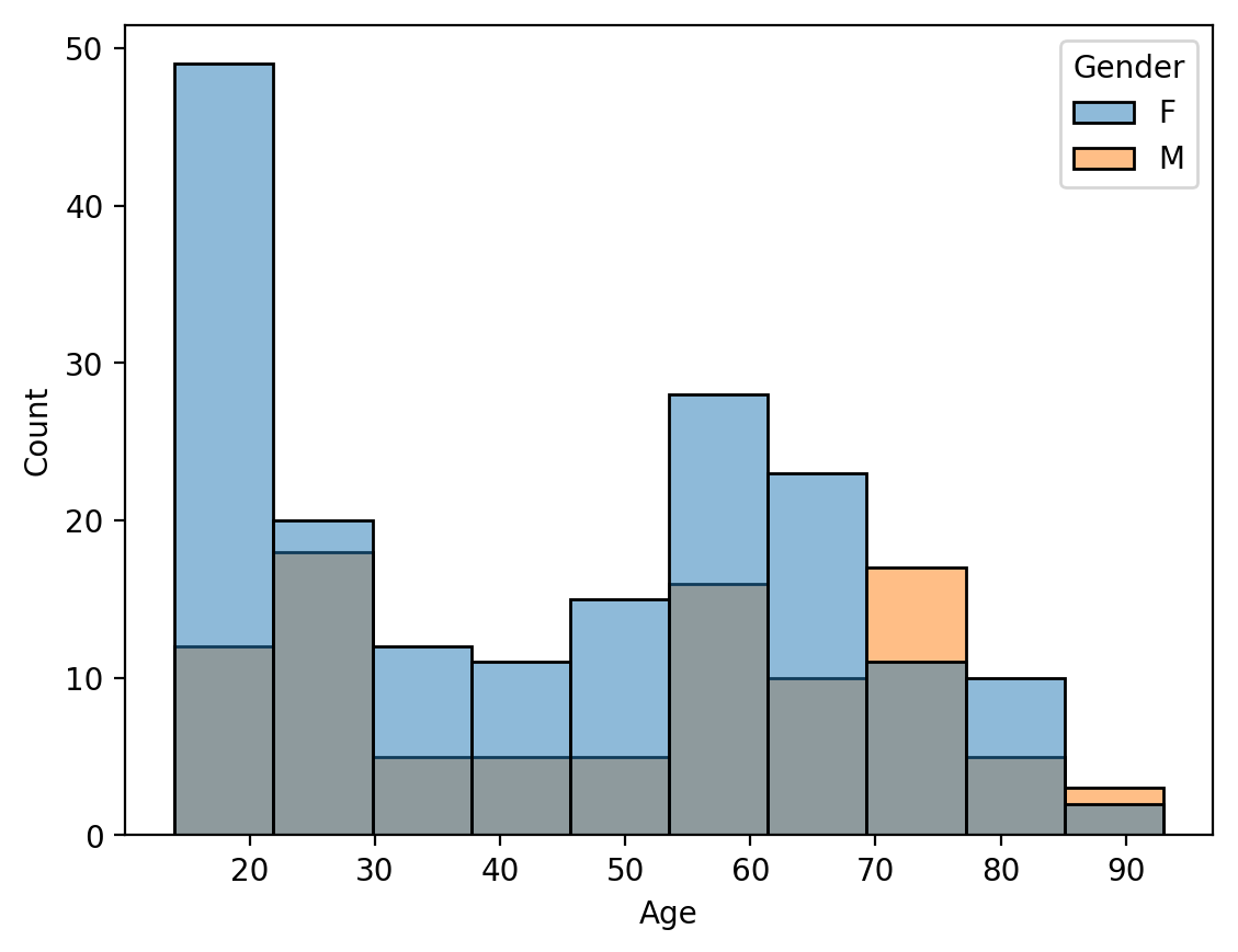
| Gender | Age | ||
|---|---|---|---|
| mean | count | ||
| 0 | F | 43.861878 | 181 |
| 1 | M | 50.020833 | 96 |
Seems like there’s about twice as many women in the dataset than men, with many of the women being younger on average.
What about the age and diagnosis breakdown?
sns.histplot(data=diagnosis_df, x="Age", hue="Diagnosis ")
plt.show()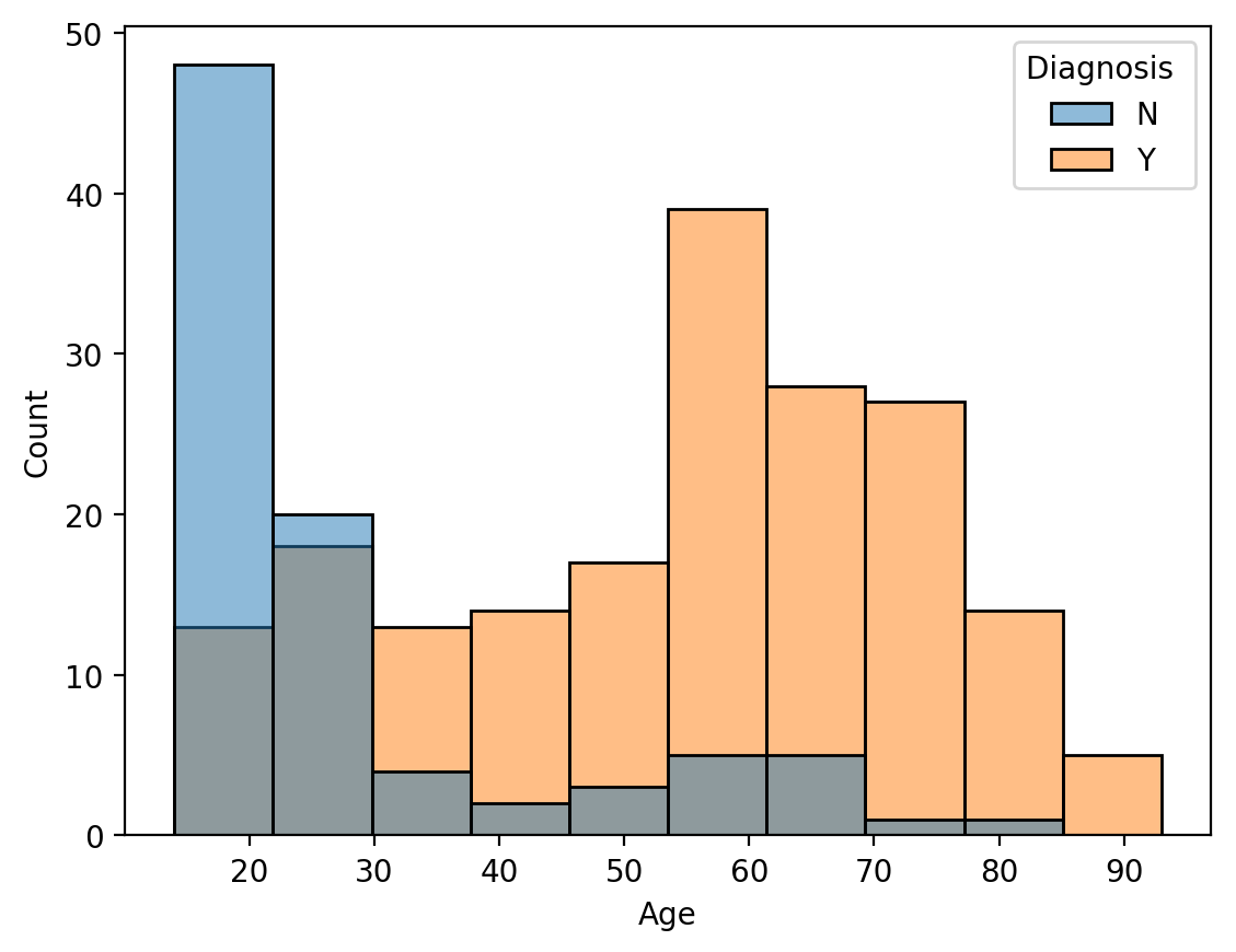
While there are quite a few young people with diagnosis, we see that healthy older individuals are underrepresented in the dataset, and the majority of those with diagnoses skew older.
From this point on, it’s important to note that I’m only dealing with the training set to avoid biasing the results we find. It is okay to compute statistics about the demographics over the entire dataset, but, since we are hoping to build models that learn the perceptual qualities, performing data exploration with them in the data could possibly bias our findings. To make sure we have a proper test set to evaluate our findings on, we’ll conduct our exploration on the training data.
Let’s go ahead and visualize the relationship between vocal health and the CAPE-V ratings as reported in the PVQD. First, we’ll compute some aggregate statistics between speakers with diagnoses and those without.
# Make sure that the diagnosis_df's File column matches that of pq_train
diagnosis_df["File"] = diagnosis_df["File"].str.upper().str.strip()
# Merge the two dataframes using a left join
matched_df = pq_train.merge(diagnosis_df, how="left", on="File")
# Filter out the NaN Examples and Run a Quick Check
matched_df = matched_df[~pd.isnull(matched_df["Gender"])]
assert len(matched_df[pd.isnull(matched_df["Gender"])]) == 0
# Here's a df of the PQs and the diagnosis value
pq_and_diagnosis_df = matched_df[["Diagnosis ", "Breathiness", "Loudness", "Pitch", "Roughness", "Strain"]]
# TODO: Calculate the Average, Median, and Max PQ per diagnosis
pq_and_diagnosis_df.groupby("Diagnosis ").agg(["mean", "median", "max"]).round(2)| Breathiness | Loudness | Pitch | Roughness | Strain | |||||||||||
|---|---|---|---|---|---|---|---|---|---|---|---|---|---|---|---|
| mean | median | max | mean | median | max | mean | median | max | mean | median | max | mean | median | max | |
| Diagnosis | |||||||||||||||
| N | 8.81 | 5.50 | 38.0 | 4.24 | 2.94 | 21.83 | 4.69 | 2.33 | 20.83 | 11.76 | 10.17 | 44.62 | 9.88 | 8.21 | 32.50 |
| Y | 24.06 | 16.17 | 99.5 | 24.49 | 14.67 | 99.17 | 22.02 | 12.17 | 99.17 | 25.78 | 21.50 | 84.83 | 26.20 | 18.17 | 96.83 |
This isn’t the prettiest table, but it gets the point across. We see the sort of trends we’d expect. Comparing means and medians across perceptual qualities, we note that voices with diagnoses have higher ratings than those without, with the maximum values for diagnosed speakers across all PQs except roughness being close to 100. If you’re familiar with statistics, you might be wondering if these differences are statistically significant. I leave it as an exercise to the reader to test this question in the associated workbooks! For this exploration, I’m happy enough to note that the difference we’d expect to see is indeed there. The max for non-diagnosed voices is lower, but can vary greatly from PQ to PQ. Breathiness, for example, has a maximum value of 38.0 while loudness has a maximum value of 21.83.
Let’s visualize the distributions to understand if these are flukes or a larger part of the distribution. Orange represents speakers without a diagnosis.
# Same df as before, but going to include the File to make it clearer
pq_and_diagnosis_df = matched_df[["File", "Age", "Diagnosis ", "Breathiness", "Loudness", "Pitch", "Roughness", "Strain"]]
# Make a Long DataFrame
long_df = pd.melt(pq_and_diagnosis_df, id_vars = ["File", "Age", "Diagnosis "], value_vars=["Breathiness", "Loudness", "Pitch", "Roughness", "Strain"], var_name = "PQ", value_name = "Value")
# Make a FacetGrid to plot a lot of things all at once
g = sns.FacetGrid(data=long_df, col = "PQ", hue = "Diagnosis ")
g.map(sns.histplot, "Value")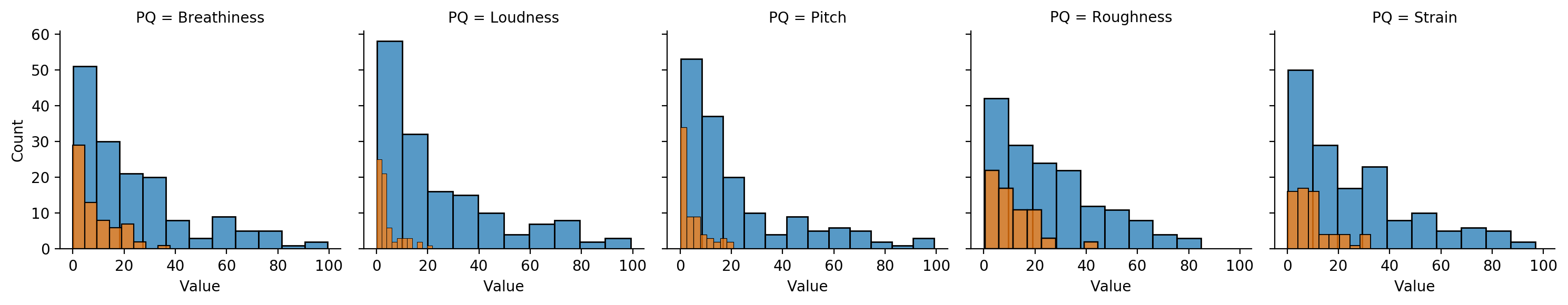
Cool! It seems like it kind of is a fluke, with the highest value being around 25-30 for many of the non-diagnosed voices. It would be good to compute different quartiles or a CDF right about now to more rigorously confirm this, but also going to leave this to the curious reader :D
We still haven’t looked at age and these perceptual qualities yet. Let’s go ahead and combine the above plots with an age dimension. Orange again represents voices without a diagnosis.
# Make a FacetGrid to plot a lot of things all at once
g = sns.FacetGrid(data=long_df, col = "PQ", hue = "Diagnosis ")
g.map(sns.scatterplot, "Age", "Value")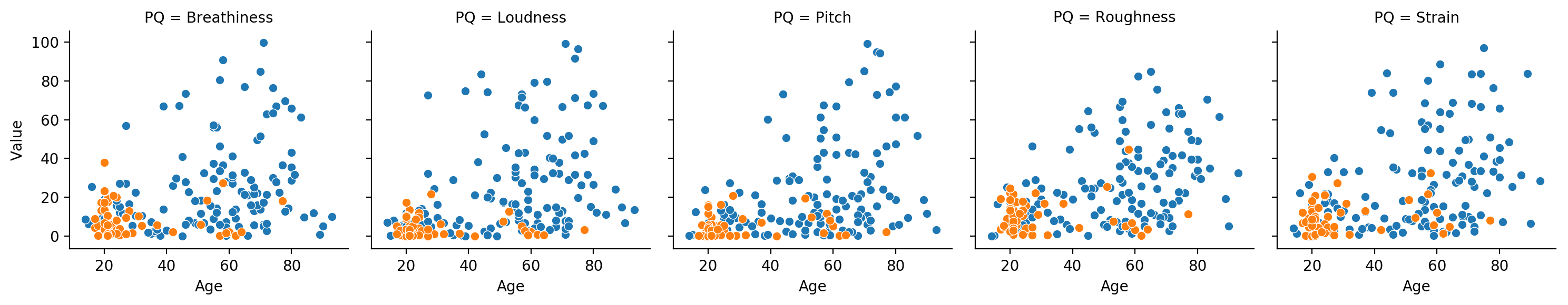
It’s interesting to note that across PQs there tends to be a slight correlation between age and the perceptual quality, with a few of the PQs, like strain, not having any examples of folks who are younger than 30 with highly strained voices. Some PQs do have examples for younger individuals, but even then it’s not many.
There’s one main takeaway we walk away with by performing this data exploration: we learn about the data distributions and correlations present in the PVQD data (under our particular set of processing choices). This can tell us about the limits of various modeling approaches we can expect, or failures of generation. For example, if we were to train a model that sought to return a 1-100 value for strain from an individual’s voice, if that individual is young and has a strained voice, our model might not be able to generalize to this new datapoint–possibly returning that the voice is less strained than it actually is. In this case, the model would have too strongly associated strain with age-specific vocal features, instead of learning what strain is across age groups. This visualization and exploration helps point out possible failures of modeling we could expect.
Another takeaway from this exploration is how SLPs label audio data ccording to the CAPE-V protocol. If we wished to incorporate different types of data, or perhaps even learn how to provide CAPE-V ratings ourselves, it’s incredibly important to know the difference between voices with high and low values of a particular perceptual quality. Given that this dataset is primarily concerned with patients with voice disorders, knowing the values that healthy or “typical” voices might have lets us know what PQ values healthy voices in other datasets should have. Generalization is a huge issue for machine learning and deep learning models. Having knowledge about how experts use the CAPE-V protocol across voices facilitates the future collection of more data to mitigate the generalization issue.
In the next post, we’re going to try to and actually model some of these perceptual qualities. Let’s see if we can do as the experts do!